The UNIQUE formula, in Excel, makes short work of removing duplicates from a list.
It comes in two main formats. You can totally remove any items that appear more than once in your list, or just keep one instance of each item from the list.
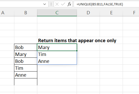
Here is an example where the duplicated items are removed completely.
Notice the Bob has been removed from the list as they appeared twice in the original list.
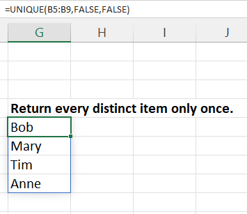
The alternative settings will return each item only once, no matter how many times it appeared in the original list. So, this time Bob is listed, but only once.
How the Unique function works
=UNIQUE(array,[by_col],[exactly_once])
array – The range that has the values you are interested in.
[by_col] -Notice the square brackets. This means the input is optional. Set to True-if your data is in different columns, otherwise put False or leave blank as this is the default.
[exactly_once] – again this is optional input: True if you want only values that occur once, the first example above, otherwise False – which is the default, the second example.
This is another example of a formula that will SPILL into other cells.