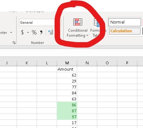
Conditional Formatting, such a great tool. On the home tab of your #Excel sheet or shortcut key Alt, H, L.
Start by selecting the cells that you want to apply the formatting too.
I have used it to highlight all the cells in my column that are over 85. You can use it to automatically highlight the top 10 values, or the lowest 5%, or cells that contain a certain word, or many other options.
The great thing is that the spreadsheet works out which cells to highlight. You can use more than one rule for any group of cells. For example, you can highlight ‘Good’ in green, ‘Ok’ in orange and ‘Bad’ in red, all without having to actually do any of the highlighting yourself. Just set the Conditional Formatting, enter your data, and the colours will appear as if by magic.
By selecting More rules… from within one of the sub-Menus under Conditional Formatting you can customise the instructions and the type of formatting.
Give it a go next time you want a particular type of data to stand out.