You can do a lot with custom number formats.
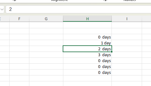
One thing that is tricky is when you are presenting information and you want to have the units correct is allowing for 0 days, 1 day, 2 days. The lack of “s” when the unit is 1 is tricky, but can be sorted with a custom number format!
To access the Custom Number Format, on the Home menu, go to the number section and click the down arrow in the selection box. Choose More Number Formats and then the Custom section. (shortcut keys Alt, H, FM.)
You can select a format that is already there and change it to suit your needs.
A number format can have up to four sections of code, separated by semicolons. These code sections define the format for positive numbers, negative numbers, zero values, and text, in that order.
<POSITIVE>;<NEGATIVE>;<ZERO>;<TEXT>
More information at https://support.microsoft.com/en-us/office/review-guidelines-for-customizing-a-number-format-c0a1d1fa-d3f4-4018-96b7-9c9354dd99f5
You can override the Positive;Negative sections by adding a condition in square brackets.

[=1]General” day”;General ” days” is the code to get our day/days showing correctly. I have added the condition, that when the value is 1, then it should be followed by “day”. Otherwise, it should be followed by “days”. The General is necessary in order to show the value as well as the day/days.
You will notice that the value in the cell is just still a number. So, you can use these numbers in calculations. The day/days is only in the formatting, it doesn’t affect the value in the cell.