A lot of users of Excel know about the filter buttons. You can read about them here: The filter function allows you to filter data into another place in your workbook, leaving your original data as is. Just like the filter buttons you can display some information from a list based on specified selection criteria.
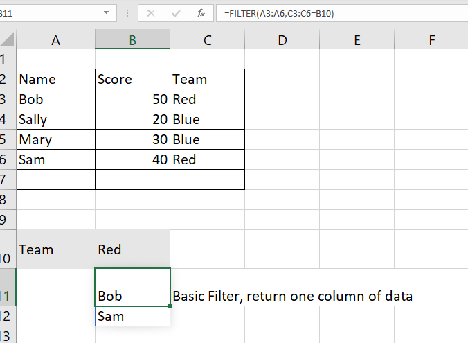
This simple FILTER function returns the names of the people from the list above that are in the team specified in B10, Red in this case.
The structure of the FILTER function is:
=FILTER(array,include,[if_empty])
Array – where is the data you are choosing from. In the case above that is the list of names from A3 to A6.
Include – Which items do you want to be returned? This must give a list that is the same length as the array. In this case we are choosing the people that are in the Red team. So, we give the list where the teams names are stored (C3 to C6) and “=B10” which has “Red” in it.
if_empty – notice the square brackets. This means the input in optional. We can tell the formula what to return if there are not items in the list to return. “Missing”, “Nothing found”, or “” (blank) would all be good options. Without this, you will get a #CALC! error if there is nothing to return.
There is a lot more detail here.
This is an example of a formula that will “SPILL” down into the cells below, so even though the formula is only in one cell, the results of the formula take up, in this case, two cells. This is indicated by the blue box.