Add Filter buttons to your data using Sort and Filter, then Filter. Found on the Home Menu. (Shortcut keys: Alt H, S, F)
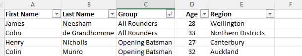
If you add filters to your data, you can access the sorting from the filter button.
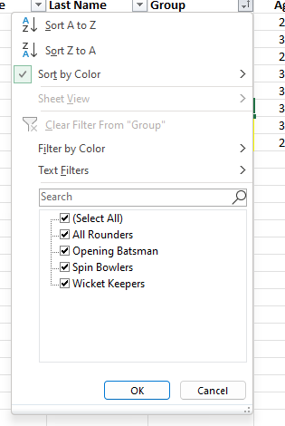
Sort A to Z (Smallest to Largest) and Z to A (Largest to Smallest) are available at the top of the drop-down list. You can also access Custom Sort by choosing the Sort by Color option, then Custom Sort.
Filtering
You can also select which rows of the data you want to see, by ticking (or unticking) the data. Once you have made a selection the row numbers on your data will be blue. This indicates that a filter is in place. The drop-down box will also change from a triangle to a filter shape on the column heading that you filtered on.
On the left-hand side of the Status Bar (at the very bottom of the sheet) it will tell you how many rows are found for that filter out of the total number of rows in your data.
You can filter by more than one column at a time. Just select the next column you want to filter by and follow the same process as before. Only the values currently showing will be available for ticking/unticking.
To turn the filter off, click the dropdown button, and choose “Clear Filter from”, or tick the (Select All) option. This will turn off the filter for that column. You will need to do that for each column you have filtered if you want to see all your data again. Alternatively, selecting Sort & Filter, then filter again will remove the filter buttons dropdowns and turn off all the filtering.