Sorting used to have to be done in place, but the Excel SORT function allows you to present data from one place, in another place sorted by your specifications.
Here is a simple example. This is a list of companies, in company order, their listings and market share. This is our original data.
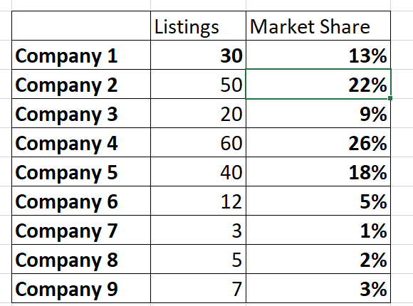
What if we want to list the companies in order of market share, highest to lowest? SORT function.
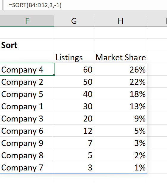
We have used one formula to sort all the information in the list into market share order.
The anatomy of the formula is: =SORT(array,[sort_index],[sort_order],[by_col])
array – Where the data to sort is. In the example above this is B4 to D12.
sort_index – note the square brackets this means this input is optional. The column number to sort by: we want market share, which is the third column of our data, so in the example above we have put 3. If you don’t put anything here, then our list will be sorted by the first column.
sort_order – Another optional input. A number that indicates the order you want: -1 for descending order in our example. (1 for ascending, or leave blank as this is the default).
by_col – Again, optional. If your data to arranged differently, and you want to sort by columns rather than rows set this to TRUE.
This is another good example of a function that SPILLS into other cells around it. Notice the blue outline around the sorted data. The formula is only actually in cell F4 but the result of the formula spills out into the surrounding cells.