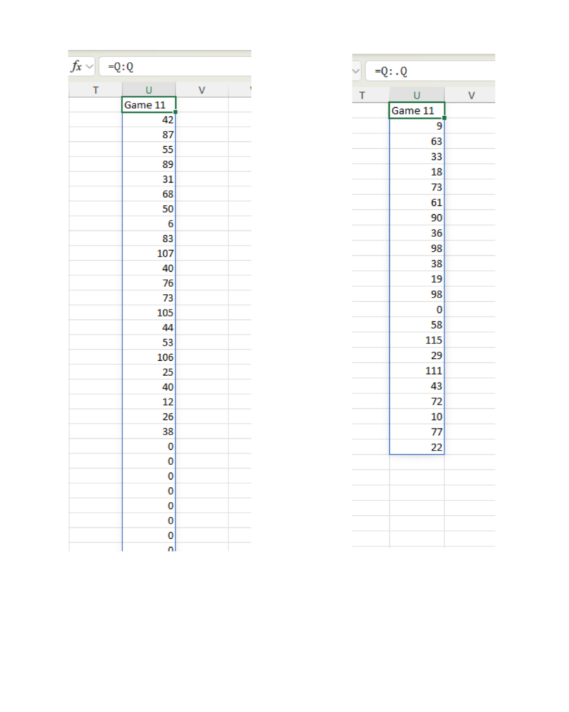
You can now reference a whole column, but not the whole column in Excel and all with a dot which stands in place for the TRIMRANGE function.
That might be a confusing statement, so let me explain. See the picture below. In both, I have referenced the whole of column Q. In the left-hand picture, the result is spilling all the way down the column and will contain a lot of zeros. In the right-hand picture only values from column Q are shown. The blank cells, which render as zero’s are not shown. And all this is achieved by the dot in front of the second Q.

You can achieve the same thing, and more with the TRIMRANGE function.
=TRIMRANGE(range,[trim_rows],[trim_cols])
| Argument | Description |
|---|---|
| rangeRequired | The range (or array) to be trimmed |
| trim_rows | Determines which rows should be trimmed0 – None1 – Trims leading blank rows2 – Trims trailing blank rows3 – Trims both leading and trailing blank rows (default) |
See here for more information.
There is a great video showing how this all works and some interesting use cases.
Now, it is worth pointing out that referencing a whole column like that has some downsides. If someone adds data there that you don’t won’t referenced, it will show up anyway. A table is usually a better way to go, but won’t work in all situations so that is when it is handy to remember TRIMRANGE.